
티스토리 뷰
반응형
주성분 분석
차원 축소
이미지 데이터는 크기가 너무 크기 때문에 디스크를 최적화하기 위해 결과에 영향을 미치지 않을 정도로 이미지의 차원을 축소해야 한다.
PCA 클래스

- PCA 알고리즘: 데이터의 분포를 가장 잘 나타내는 주성분(선)을 이용하는 알고리즘
- 주성분은 여러 개가 존재할 수도 있다. 차원 축소를 통해 주성분의 개수를 줄일 수 있다.
- 주성분은 기존 주성분의 수직 방향으로 차례대로 찾는다.
데이터 준비하기
!wget https://bit.ly/fruits_300_data -O fruits_300.npyimport numpy as np
fruits = np.load('fruits_300.npy')
fruits_2d = fruits.reshape(-1, 100*100)
PCA 클래스를 이용해 먼저 50개의 주성분만 찾도록 한다.
from sklearn.decomposition import PCA

# 50개의 주성분만 찾도록 함
pca = PCA(n_components=50)
pca.fit(fruits_2d)

# 주성분이 가지는 속성은 10000개
print(pca.components_.shape)
# 결과
(50, 10000)
plt 모듈로 각 그림의 주성분을 이미지로 출력해보자.
import matplotlib.pyplot as plt

def draw_fruits(arr, ratio=1):
  n = len(arr)
  rows = int(np.ceil(n/10))
  cols = n if rows < 2 else 10
  fig, axs = plt.subplots(rows, cols,
                          figsize=(cols*ratio, rows*ratio), squeeze=False)

  for i in range(rows):
    for j in range(cols):
      if i*10 + j < n:
        axs[i, j].imshow(arr[i*10 + j], cmap='gray_r')
      axs[i, j].axis('off')
  plt.show()


draw_fruits(pca.components_.reshape(-1, 100, 100))print(fruits_2d.shape)# 결과
(300, 10000)
이전에는 reshape 메소드를 사용했다면, PCA 클래스에서는 transform 메소드로 데이터 차원을 축소할 수도 있다.
# 데이터 차원 축소
fruits_pca = pca.transform(fruits_2d)

print(fruits_pca.shape)
# 결과
(300, 50)
원본 데이터 재구성
데이터를 이미지로 출력한 다음 확인하기 위해 색을 반전시켜주도록 하자.
fruits_inverse = pca.inverse_transform(fruits_pca)
print(fruits_inverse.shape)
# 결과
(300, 10000)
그리고 이미지 출력을 위해 1차원 데이터를 100 * 100의 2차원 데이터로 변환한다.
# 이미지로 출력하기 위해 100 * 100으로 변경
fruits_reconstruct = fruits_inverse.reshape(-1, 100, 100)

for start in [0, 100, 200]:
    draw_fruits(fruits_reconstruct[start:start+100])
    print("\n")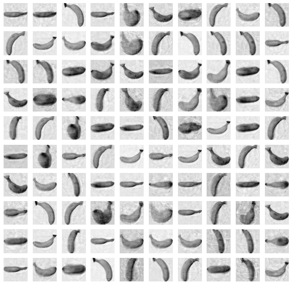
설명된 분산
각 주성분이 갖고 있는 분산을 출력해보자.
# explained_variance_ratio_ : 각 주성분이 얼마만큼의 분산을 표현하는지.
print(np.sum(pca.explained_variance_ratio_))
# 결과
0.9215186216784217
분산 값을 그래프로 수치화해보도록 한다.
plt.plot(pca.explained_variance_ratio_)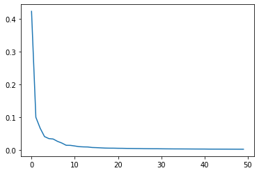
다른 알고리즘과 함께 사용하기
분류기와 함께 사용하기
from sklearn.linear_model import LogisticRegression
from sklearn.model_selection import cross_validate

lr = LogisticRegression()

target = np.array([0] * 100 + [1] * 100 + [2] * 100)

scores = cross_validate(lr, fruits_2d, target)
print(np.mean(scores['test_score']))
print(np.mean(scores['fit_time']))      # 분류하는데 걸린 시간
# 결과
0.9966666666666667
0.7837676525115966
PCA를 함께 사용했을 때 fit time이 훨씬 줄어들었다.
scores = cross_validate(lr, fruits_pca, target)
print(np.mean(scores['test_score']))
print(np.mean(scores['fit_time']))
# 결과
1.0
0.034157514572143555
PCA 클래스의 주성분 개수는 2개가 적합하다.
pca = PCA(n_components=0.5)
pca.fit(fruits_2d)

# 2개의 주성분만 있으면 충분
print(pca.n_components_)
# 결과
2
군집과 함께 사용하기
from sklearn.cluster import KMeans

km = KMeans(n_clusters=3, random_state=42)
km.fit(fruits_pca)

print(np.unique(km.labels_, return_counts=True))
# 결과
(array([0, 1, 2], dtype=int32), array([110, 99, 91]))
시각화
이전에 사용한 주성분 2개를 2차원 그래프 위에 그려 시각화해볼 수 있다.
for label in range(0, 3):
    data = fruits_pca[km.labels_ == label]
    plt.scatter(data[:,0], data[:,1])
plt.legend(['apple', 'banana', 'pineapple'])
plt.show()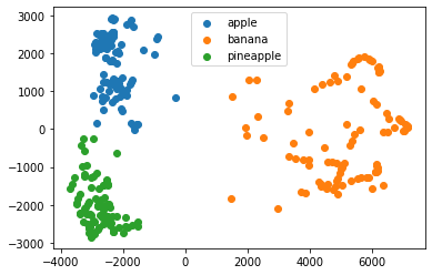
반응형
'ML' 카테고리의 다른 글
| 혼자 공부하는 머신러닝 + 딥러닝 7장 심층 신경망 리뷰 (0) | 2022.06.12 |
|---|---|
| 혼자 공부하는 머신러닝 + 딥러닝 7장 인공 신경망 리뷰 (0) | 2022.06.10 |
| 혼자 공부하는 머신러닝 + 딥러닝 6장 K-평균 리뷰 (0) | 2022.06.10 |
| 혼자 공부하는 머신러닝 + 딥러닝 6장 군집 알고리즘 리뷰 (0) | 2022.06.10 |
| 혼자 공부하는 머신러닝 + 딥러닝 5장 리뷰 (0) | 2022.05.04 |
공지사항
최근에 올라온 글
최근에 달린 댓글
- Total
- Today
- Yesterday
링크
TAG
- virtualbox
- baekjoon
- linuxgedit
- whatis
- 버추억박스에러
- cat
- 버추억박스오류
- linux파일
- GithubAPI
- atq
- 코테
- linuxawk
- cron시스템
- Baekjoon27219
- 백준27211
- awk프로그램
- Baekjoon27211
- linuxtouch
- 리눅스cron
- GitHubAPIforJava
- 백준
- 리눅스
- OnActivityForResult
- api문서
- E_FAIL
- SELECT #SELECTFROM #WHERE #ORDERBY #GROUPBY #HAVING #EXISTS #NOTEXISTS #UNION #MINUS #INTERSECTION #SQL #SQLPLUS
- 사용자ID
- Linux
- 쇼미더코드
- 백준27219
| 일 | 월 | 화 | 수 | 목 | 금 | 토 |
|---|---|---|---|---|---|---|
| 1 | 2 | 3 | 4 | 5 | ||
| 6 | 7 | 8 | 9 | 10 | 11 | 12 |
| 13 | 14 | 15 | 16 | 17 | 18 | 19 |
| 20 | 21 | 22 | 23 | 24 | 25 | 26 |
| 27 | 28 | 29 | 30 |
글 보관함